If You are a R Developer, Then You Must Try SAP HANA for Free.

This is a guest blog from Alvaro Tejada Galindo, my colleague and fellow R and SAP HANA enthusiast.  I am thankful to Alvaro for coming and posting on "AllThingsBusinessAnalytics".

Are you an R developers? Have ever heard of SAP HANA? Would you like to test SAP HANA for free?

SAP HANA is an In-Memory Database Technology allowing developers to analyze big data in real-time.

Processes that took hours now take seconds due to SAP HANA's power to keep everything on RAM memory.

As announced in SAP Sapphire Now event in Orlando, Florida, SAP HANA is free for developers. You just need to download and install both the SAP HANA Client and the SAP HANA Studio, and create an SAP HANA Server on the Amazon Web Services as described in the following document:

Get your own SAP HANA DB server on Amazon Web Services - http://scn.sap.com/docs/DOC-28294

Why should this interest you? Easy...SAP HANA is an agent of change bringing speed to its limits and it can also be integrated with R as described in the following blog:

When SAP HANA met R - First kiss - http://scn.sap.com/community/developer-center/hana/blog/2012/05/21/when-sap-hana-met-r--first-kiss

Want to know more about SAP HANA? Read everything you need here: http://developers.sap.com

You're convinced but don't want to pay for the Amazon Web Services? No problem. Just leave a comment including your name, company and email. We will reach you and send you an Amazon Gift Card so you can get started. Of course, your feedback would be greatly appreciated. Of course, we only a limited set of gift cards, so be quick or be out.

Author Alvaro Tejada Galindo, mostly known as "Blag" is a Development Expert working for the Technology Innovation and Developer Experience team in SAP Labs.  He can be contacted at a.tejada.galindo@sap.com.

Alvaro's background in his own words: I used to be an ABAP Consultant for 11 years. I worked in implementations on Peru and Canada. I’m also a die hard developer using R, Python, Ruby, PHP, Flex and many more languages. Now, I work for SAP Labs and my main roles are evangelize SAP technologies by writing blogs, articles, helping people on the forums, attending SAP events, besides many other “Developer engagement” activities.

I maintain a blog called “Blag’s bag of rants” at blagrants.blogspot.com

Why Delta's Foray into the Crude Refining Business is a BAD Move?

When my mentor/guide and company president Sanjay Poonen threw this open challenge on Twitter:

Sanjay Poonen ‏ @spoonen

For all u MBAs, what do u think of Delta buying an oil refinery for $150M (formerly $1B) for top-grade jet fuel. Would Michael Porter frown?

how could I have passed on this challenge PLUS I have been lately descending deep into the technology roots (most of my blogs are technical with lots of code snippets for all intentional purposes - AllThingsR.)  So I decided to spend some time sleuthing and analyzing hard facts before replying to @spoonen, and (may be) counter @gkm1 (George Mathew's) arguments.  This way I get back into analyzing business topics for some time.  (After all, A in MBA stands for analysis right? Masters in Business Analytics?)

The original news on WSJ covering Delta decision to buy a refinery from ConocoPhillips is here.

I spent quite sometime researching so I can educate myself on this deal.  I started with a prior belief that this is a BAD deal.  After all, the crude refining business is a boom and bust business, has razor thin margins and is notoriously competitive.  Here is a quote from Bloomberg supporting my argument: "Refiners in the northeastern U.S. are struggling to turn a profit because of the narrow margin between the cost of imported crude and fuel prices." (Source: Bloomberg)

Moreover, not a single new refinery has sprung up in the US for at least 35 years (Source) because no one wants to invest in this business.  In addition, ConocoPhillips, had idled this refinery for few months now and Sunoco, another refiner in that area, is in the process of shutting down two more refineries in that region. (Source: Bloomberg)  "Sunoco...said its refining businesses has been losing $1 million dollars a day for three years running." (Source)

So why is Delta buying this refinery? Vertical integration, fuel hedging, cost-savings, political, EPS improvements etc?  Actually all of the above.

Delta's planes burned 3.9B gallons of jet fuel last year.  At an avg. 2011 price of $2.86 per gallon, Delta spent $11.8B, which is 40% of its operating expenses. (Source: NYTimes)  If the cost of jet fuel was 40% of your company's operating expense, you will also be thinking about taking such dramatic decisions but may not execute on it if it is outside your realm, but Delta did.

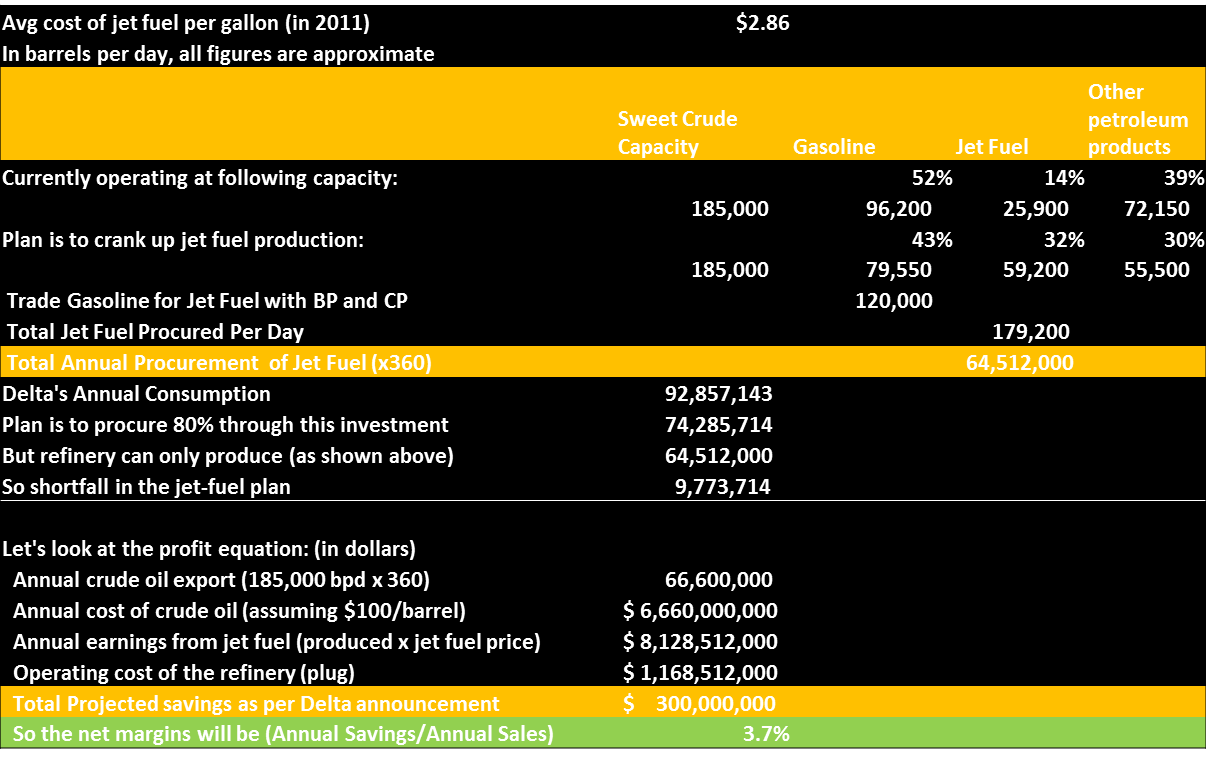
Delta will pay $150M in cash (it has $3B in cash on its balance sheet, so there is no liquidity issue) and will invest another $100M in retooling this refinery.  Also you should note that PA government is chipping in with additional $30M (Thank you tax payers!).  Retooling is required for reason self-evident in this table (Mainly to crank-up the jet-fuel production):

Now, looking at this table why would anyone believe that Delta can earn $300M every year from this. Also remember, Delta is not bringing down its fuel cost from ~$12B by a whole lot, it is merely trying to save few cents on the dollar. A little bit of shift in the numbers above and Delta will be in red trouble.

Delta said that this is a good deal for the investors, really?  Valero had margins of less than 3% in its last quarter and it is a pure play refinery company. Can Delta beat Valero on margins?  I have my serious doubts.  This could be a gain but just for the Delta's management as it attempts to boost EPS in the near-term.

Also, can you believe that Delta can really retool the refinery and produce more jet-fuel than it is possible? The bio-chemistry doesn't support it.  From one barrel of crude, only 19.5 gallons of gasoline and 4.1 gallons of  jet-fuel can be produced.  How is Delta going to produce more jet-fuel per barrel of crude?

Also, FYI, this refinery can only process light sweet crude (with low sulfur) not that heavy Saudi oil that has high sulfur and is gaining more prominence due to global oil issues. (Source: ConocoPhillips)

Net net, this is a bad move, Delta will burn itself and get out in a year or two.  And when they sell, it will be a fire, sale since many other refineries in that area are already struggling to make a profit as I mentioned above. Delta's thinking that future of refineries is brighter is quite puzzling for me.

Happy Analyzing!

Big Data, R and SAP HANA: Analyze 200 Million Data Points and Later Visualize in HTML5 Using D3 - Part III

Mash-up Airlines Performance Data with Historical Weather Data to Pinpoint Weather Related Delays

For this exercise, I combined following four separate blogs that I did on BigData, R and SAP HANA.  Historical airlines and weather data were used for the underlying analysis. The aggregated output of this analysis was outputted in JSON which was visualized in HTML5, D3 and Google Maps.  The previous blogs on this series are:

1. Big Data, R and HANA: Analyze 200 Million Data Points and Later Visualize in HTML5 Using D3 - Part II
2. Big Data, R and HANA: Analyze 200 Million Data Points and Later Visualize Using Google Maps
3. Getting Historical Weather Data in R and SAP HANA 
4. Tracking SFO Airport's Performance Using R, HANA and D3

In this blog, I wanted to mash-up disparate data sources in R and HANA by combining airlines data with weather data to understand the reasons behind the airport/airlines delay.  Why weather - because weather is one of the commonly cited reasons in the airlines industry for flight delays.  Fortunately, the airlines data breaks up the delay by weather, security, late aircraft etc., so weather related delays can be isolated and then the actual weather data can be mashed-up to validate the airlines' claims.  However, I will not be doing this here, I will just be displaying the mashed-up data.

I have intentionally focused on the three bay-area airports and have used last 4 years of historical data to visualize the airport's performance using a HTML5 calendar built from scratch using D3.js.  One can use all 20 years of data and for all the airports to extend this example.  I had downloaded historical weather data for the same 2005-2008 period for SFO and SJC airports as shown in my previous blog (For some strange reasons, there is no weather data for OAK, huh?).  Here is how the final result will look like in HTML5:

Click here to interact with the live example.  Hover over any cell in the live example and a tool tip with comprehensive analytics will show the break down of the performance delay for the selected cell including weather data and correct icons* - result of a mash-up.  Choose a different airport from the drop-down to change the performance calendar. 

* Weather icons are properties of Weather Underground.

As anticipated, SFO airport had more red on the calendar than SJC and OAK.  SJC definitely is the best performing airport in the bay-area.  Contrary to my expectation, weather didn't cause as much havoc on SFO as one would expect, strange?

Creating a mash-up in R for these two data-sets was super easy and a CSV output was produced to work with HTML5/D3.  Here is the R code and if it not clear from all my previous blogs: I just love data.table package.

###########################################################################################  

# Percent delayed flights from three bay area airports, a break up of the flights delay by various reasons, mash-up with weather data

###########################################################################################  

baa.hp.daily.flights <- baa.hp[,list( TotalFlights=length(DepDelay), CancelledFlights=sum(Cancelled, na.rm=TRUE)), 

                             by=list(Year, Month, DayofMonth, Origin)]

setkey(baa.hp.daily.flights,Year, Month, DayofMonth, Origin)

baa.hp.daily.flights.delayed <- baa.hp[DepDelay>15,

                                     list(DelayedFlights=length(DepDelay), 

                                      WeatherDelayed=length(WeatherDelay[WeatherDelay>0]),

                                      AvgDelayMins=round(sum(DepDelay, na.rm=TRUE)/length(DepDelay), digits=2),

                                      CarrierCaused=round(sum(CarrierDelay, na.rm=TRUE)/sum(DepDelay, na.rm=TRUE), digits=2),

                                      WeatherCaused=round(sum(WeatherDelay, na.rm=TRUE)/sum(DepDelay, na.rm=TRUE), digits=2),

                                      NASCaused=round(sum(NASDelay, na.rm=TRUE)/sum(DepDelay, na.rm=TRUE), digits=2),

                                      SecurityCaused=round(sum(SecurityDelay, na.rm=TRUE)/sum(DepDelay, na.rm=TRUE), digits=2),

                                      LateAircraftCaused=round(sum(LateAircraftDelay, na.rm=TRUE)/sum(DepDelay, na.rm=TRUE), digits=2)), by=list(Year, Month, DayofMonth, Origin)]

setkey(baa.hp.daily.flights.delayed, Year, Month, DayofMonth, Origin)

# Merge two data-tables

baa.hp.daily.flights.summary <- baa.hp.daily.flights.delayed[baa.hp.daily.flights,list(Airport=Origin,

                           TotalFlights, CancelledFlights, DelayedFlights, WeatherDelayed, 

                           PercentDelayedFlights=round(DelayedFlights/(TotalFlights-CancelledFlights), digits=2),

                           AvgDelayMins, CarrierCaused, WeatherCaused, NASCaused, SecurityCaused, LateAircraftCaused)]

setkey(baa.hp.daily.flights.summary, Year, Month, DayofMonth, Airport)

# Merge with weather data

baa.hp.daily.flights.summary.weather <-baa.weather[baa.hp.daily.flights.summary]

baa.hp.daily.flights.summary.weather$Date <- as.Date(paste(baa.hp.daily.flights.summary.weather$Year, 

                                                           baa.hp.daily.flights.summary.weather$Month, 

                                                           baa.hp.daily.flights.summary.weather$DayofMonth, 

                                                           sep="-"),"%Y-%m-%d")

# remove few columns

baa.hp.daily.flights.summary.weather <- baa.hp.daily.flights.summary.weather[, 

            which(!(colnames(baa.hp.daily.flights.summary.weather) %in% c("Year", "Month", "DayofMonth", "Origin"))), with=FALSE]

#Write the output in both JSON and CSV file formats

objs <- baa.hp.daily.flights.summary.weather[, getRowWiseJson(.SD), by=list(Airport)]

# You have now (Airportcode, JSONString), Once again, you need to attach them together.

row.json <- apply(objs, 1, function(x) paste('{\"AirportCode\":"', x[1], '","Data\":', x[2], '}', sep=""))

json.st <- paste('[', paste(row.json, collapse=', '), ']')

writeLines(json.st, "baa-2005-2008.summary.json")                 

write.csv(baa.hp.daily.flights.summary.weather, "baa-2005-2008.summary.csv", row.names=FALSE)

Happy Coding!

Big Data, R and SAP HANA: Analyze 200 Million Data Points and Later Visualize in HTML5 Using D3 - Part II

Technologies: SAP HANA, R, HTML5, D3, JQuery and JSON

In my last blog, Big Data, R and SAP HANA: Analyze 200 Million Data Points and Later Visualize Using Google Maps, I analyzed historical airlines performance data set using R and SAP HANA and put the aggregated analysis on Google Maps.  Undoubtedly, Map is a pretty exciting canvas to view and analyze big data sets. One could draw shapes (circles, polygons) on the map under a marker pin, providing pin-point information and display aggregated information in the info-window when a marker is clicked.  So I enjoyed doing all of that, but I was craving for some old fashion bubble charts and other types of charts to provide comparative information on big data sets.  Ultimately, all big data sets get aggregated into smaller analytical sets for viewing, sharing and reporting.  An old fashioned chart is the best way to tell a visual story!

On bubble charts, one could display 4 dimensional data for comparative analysis. In this blog analysis, I used the same data-set which had 200M data points and went deeper looking at finer slices of information.  I leveraged D3, R and SAP HANA for this blog post.  Here I am publishing some of this work:  

In this first graphics, the performance of top airlines is compared for 2008.  As expected, Southwest, the largest airlines (when using total number of flights as a proxy), performed well for its size (1.2M flights, 64 destinations but average delay was ~10 mins.)  Some of the other airlines like American and Continental were the worst performers along with Skywest.  Note, I didn't remove outliers from this analysis.  Click here to interact with this example.

In the second analysis, I replaced airlines dimension with airports dimension but kept all the other dimensions the same.  To my disbelief, Newark airport is the worst performing airport when it comes to departure delays.  Chicago O'Hare, SFO and JFK follow.  Atlanta airport is the largest airport but it has the best performance. What are they doing differently at ATL?  Click here to interact with this example.

It was hell of a fun playing with D3, R and HANA, good intellectual stimulation if nothing else!  Happy Analyzing and remember possibilities are endless!

As always, my R modules are fairly simple and straightforward:
###########################################################################################  
#ETL - Read the AIRPORT Information, get major aiport informatoin extracted and upload this 
#transfromed dataset into HANA
###########################################################################################
major.airports <- data.table(read.csv("MajorAirports.csv",  header=TRUE, sep=",", stringsAsFactors=FALSE))
setkey(major.airports, iata)


all.airports <- data.table(read.csv("AllAirports.csv",  header=TRUE, sep=",", stringsAsFactors=FALSE)) 
setkey(all.airports, iata)


airports.2008.hp <- data.table(read.csv("2008.csv",  header=TRUE, sep=",", stringsAsFactors=FALSE)) 
setkey(airports.2008.hp, Origin, UniqueCarrier)


#Merge two datasets
airports.2008.hp <- major.airports[airports.2008.hp,]


###########################################################################################  
# Get airport statisitics for all airports
###########################################################################################
airports.2008.hp.summary <- airports.2008.hp[major.airports,     
    list(AvgDepDelay=round(mean(DepDelay, na.rm=TRUE), digits=2),
    TotalMiles=prettyNum(sum(Distance, na.rm=TRUE), big.mark=","),
    TotalFlights=length(Month),
    TotalDestinations=length(unique(Dest)),
    URL=paste("http://www.fly", Origin, ".com",sep="")), 
                    by=list(Origin)][order(-TotalFlights)]
setkey(airports.2008.hp.summary, Origin)
#merge two data tables
airports.2008.hp.summary <- major.airports[airports.2008.hp.summary, 
                                                     list(Airport=airport, 
                                                          AvgDepDelay, TotalMiles, TotalFlights, TotalDestinations, 
                                                          Address=paste(airport, city, state, sep=", "), 
                                                          Lat=lat, Lng=long, URL)][order(-TotalFlights)]




airports.2008.hp.summary.json <- getRowWiseJson(airports.2008.hp.summary)
writeLines(airports.2008.hp.summary.json, "airports.2008.hp.summary.json")                 
write.csv(airports.2008.hp.summary, "airports.2008.hp.summary.csv", row.names=FALSE)

Big Data, R and HANA: Analyze 200 Million Data Points and Later Visualize Using Google Maps

Technologies: SAP HANA, R, HTML5, D3, Google Maps, JQuery and JSON

For this fun exercise, I analyzed more than 200 million data points using SAP HANA and R and then brought in the aggregated results in HTML5 using D3, JSON and Google Maps APIs.  The 2008 airlines data is from the data expo and I have been using this entire data set (123 million rows and 29 columns) for quite sometime. See my other blogs

The results look beautiful:

Each airport icon is clickable and when clicked displays an info-window describing the key stats for the selected airport:

I then used D3 to display the aggregated result set in the modal window (light box):

Unfortunately, I can't provide the live example due to the restrictions put in by Google Maps APIs and I am approaching my free API limits.

Fun fact:  The Atlanta airport was the largest airport in 2008 on many dimensions: Total Flights Departed, Total Miles Flew, Total Destinations.  It also experienced lower average departure delay in 2008 than Chicago O'Hare. I always thought Chicago O'Hare is the largest US airport.

As always, I just needed 6 lines of R code including two lines of code to write data in JSON and CSV files:

################################################################################
airports.2008.hp.summary <- airports.2008.hp[major.airports,     
    list(AvgDepDelay=round(mean(DepDelay, na.rm=TRUE), digits=2),
    TotalMiles=prettyNum(sum(Distance, na.rm=TRUE), big.mark=","),
    TotalFlights=length(Month),
    TotalDestinations=length(unique(Dest)),
    URL=paste("http://www.fly", Origin, ".com",sep="")), 
                    by=list(Origin)][order(-TotalFlights)]
setkey(airports.2008.hp.summary, Origin)
#merge the two data tables
airports.2008.hp.summary <- major.airports[airports.2008.hp.summary, 
                                                     list(Airport=airport, 
                                                          AvgDepDelay, TotalMiles, TotalFlights, TotalDestinations, 
                                                          Address=paste(airport, city, state, sep=", "), 
                                                          Lat=lat, Lng=long, URL)][order(-TotalFlights)]


airports.2008.hp.summary.json <- getRowWiseJson(airports.2008.hp.summary)
writeLines(airports.2008.hp.summary.json, "airports.2008.hp.summary.json")                 
write.csv(airports.2008.hp.summary, "airports.2008.hp.summary.csv", row.names=FALSE)
##############################################################################

Happy Coding and remember the possibilities are endless!

Tracking SFO Airport's Performance Using R, HANA and D3

Visualize Big Data Using R, HANA, D3, JSON and HTML5/JavaScript

This is my first introduction to D3 and I am simply blown away.  Mike Bostock (@mbostock), you are genius and thanks for creating D3!  With HANA, R, D3, HTML5 and iPad, and you got yourself a KILLER combo!

I have been burning my midnight oil on piecing together my big data story using HANA, R, JSON and HTML5.  If you recall, I did a technical session on R and SAP HANA at DKOM, SAP's Development Kickoff Event last week where I showcased the supreme powers of R and HANA when analyzing 124 million records in real time.  R and SAP HANA: A Highly Potent Combo for Real Time Analytics on Big Data

Since last week, I have been looking for other creative ways to analyze and then visualize this airlines data. I am very fortunate to come across D3.  After spending couple of hours with D3, I decided to build the calendar view for the airlines data I have.  The calendar view is the first example Mike shows on his D3 page. Amazingly awesome!

I created this calendar view capturing the percent of delayed flight from SFO airports that departed daily between 2005-2008.  For this analysis, I used HANA to get the data out for SFO (out of 250 plus airports) over this 4 years period in seconds and then did all the aggregation in R including creating a JSON and .CSV file in seconds again.  Later, I moved to HTML5 and D3 to generate this beautiful calendar view showing SFO's performance.  Graphics is presented below:

As expected, December and January are two notorious months for flights delay.  Have fun with the live example hosted in the Amazon cloud..

Once again, my R code is very simple:


## Depature Delay for SF Airport
ba.hp.sfo <- ba.hp[Origin=="SFO",]


ba.hp.sfo.daily.flights <- ba.hp.sfo[,list(DailyFlights=length(DepDelay)), by=list(Year, Month, DayofMonth)][order(Year,Month,DayofMonth)]
ba.hp.sfo.daily.flights.delayed <- ba.hp.sfo[DepDelay>15,list(DelayedDailyFlights=length(DepDelay)), by=list(Year, Month, DayofMonth)][order(Year,Month,DayofMonth)]
setkey(ba.hp.sfo.daily.flights.delayed, Year, Month, DayofMonth)
response <- ba.hp.sfo.daily.flights.delayed[ba.hp.sfo.daily.flights]
response <- response[,list(Date=as.Date(paste(Year, Month, DayofMonth, sep="-"),"%Y-%m-%d"), 
                           #DailyFlights,DelayedDailyFlights,
                           PercentDelayedFlights=round((DelayedDailyFlights/DailyFlights), digits=2))]
objs <- apply(response, 1, toJSON)
res <- paste('{"dailyFlightStats": [', paste(objs, collapse=', '), ']}')
writeLines(res, "dailyFlightStatsForSFO.json")                 
write.csv(response, "dailyFlightStatsForSFO.csv", row.names=FALSE)


For D3 and HTML code, please take a look at this example from D3 website. 

Happy Analyzing and Keep That Mid Night Oil Burning!

Geocode and reverse geocode your data using, R, JSON and Google Maps' Geocoding API

(Reposting the previous blog with additional module on reverse geocoding added here.)

First and foremost, I absolutely love the topic of Location Analytics (Geo-Spatial Analysis) and see tremendous business potential in not so distant future.  I would go out on a limb to predict that the Location Analytics will soon go viral in the enterprise space because it has the capability to WOW us. Look no further than your iPhone or an Android phone and count how many location aware apps you have. We all have at lease one app - Google Maps.  Mobile is one of the strongest catalyst for enterprise adoption of Location aware apps. All right, enough of business talk, let's get dirty with the code.

Over the last year and half, I have faced numerous challenges with geocoding and reverse geocoding the data that I have used to showcase my passion for location analytics.  In 2012, I decided to take thing in my control and turned to R.  Here, I am sharing a simple R script that I wrote to geo-code my data whenever I needed it, even BIG Data.

To geocode and reverse geocode my data, I use Google's Geocoding service which returns the geocoded data in a JSON. I will recommend that you register with Google Maps API and get a key if you have large amount of data and would do repeated geo coding.

Geocode:

getGeoCode <- function(gcStr)  {

  library("RJSONIO") #Load Library

  gcStr <- gsub(' ','%20',gcStr) #Encode URL Parameters

 #Open Connection

 connectStr <- paste('http://maps.google.com/maps/api/geocode/json?sensor=false&address=',gcStr, sep="") 

  con <- url(connectStr)

  data.json <- fromJSON(paste(readLines(con), collapse=""))

  close(con)

  #Flatten the received JSON

  data.json <- unlist(data.json)

  if(data.json["status"]=="OK")   {

    lat <- data.json["results.geometry.location.lat"]

    lng <- data.json["results.geometry.location.lng"]

    gcodes <- c(lat, lng)

    names(gcodes) <- c("Lat", "Lng")

    return (gcodes)

  }

}

geoCodes <- getGeoCode("Palo Alto,California")

> geoCodes
           Lat            Lng 
  "37.4418834" "-122.1430195" 

Reverse Geocode:

reverseGeoCode <- function(latlng) {

latlngStr <-  gsub(' ','%20', paste(latlng, collapse=","))#Collapse and Encode URL Parameters

  library("RJSONIO") #Load Library

  #Open Connection

  connectStr <- paste('http://maps.google.com/maps/api/geocode/json?sensor=false&latlng=',latlngStr, sep="")

  con <- url(connectStr)

  data.json <- fromJSON(paste(readLines(con), collapse=""))

  close(con)

  #Flatten the received JSON

  data.json <- unlist(data.json)

  if(data.json["status"]=="OK")

    address <- data.json["results.formatted_address"]

  return (address)

}

address <- reverseGeoCode(c(37.4418834, -122.1430195))

> address
                    results.formatted_address 
"668 Coleridge Ave, Palo Alto, CA 94301, USA" 

Happy Coding!

R and SAP HANA: A Highly Potent Combo for Real Time Analytics on Big Data

Lets Talk Code

SAP DKOM 2012 kicks off in San Jose today and I can’t be more excited than this.  For the past three months Jens Doerpmund, Chief Development Architect of Analytics at SAP and I have been working on this topic of R and SAP HANA and all our hard work (upwards of 400 hours) is about to pay off (fingers crossed).

It has been a stunning journey and an incredible learning experience. Both R and HANA are fascinating technologies and bringing them together is analogous to bringing Google and Apple together. We are gearing up for our session and in the true spirit of DKOM, we will be only talking code, yes code and lots of it.  We just wrapped up our slides with lots of code snippets to share with fellow DKOMers.  Here is a quick sneak preview of what we are going to cover today:

Big Data Analytics (Really Big)

• Airlines sector in the travel industry
• 22 years (1987-2008) of airlines on time performance data on US airlines
• 123 million records
• Extract Transform Load – ETL work to combine this data with data on airports, data on carriers with this data to setup for Big Data analysis in R and HANA
• D20 with 96GB of RAM and 24 Cores
• Massive amount of data crunching using R and HANA

 We will be covering lots and lot of topics, here is a short list:

• Sentiment Analysis on #DKOM and a WordCloud
• Cluster Analysis using K-Mean
• Geo Code Your Data – Google Maps API
• SP100 - XML Parsing and Historical Stock Data
• R and HANA integration
• Moving big-data from one HANA to another HANA (Replication)
• Server side Java Scripting
• and an HTML5 App built with R, HANA and Server Side Java Script

Here is a wordcloud straight from R on #DKOM. There will be lot more to discuss today. Looking forward to meeting you all DKOMers.

Lets Talk Code Everyone and Happy Coding!

 Jitender Aswani

 Jens Doerpmund

Learn more on this session topic in my previous blog:  Advance Analytics with R and HANA at DKOM 2012 San Jose

Advanced Analytics with R and HANA at DKOM 2012 San Jose

Advanced Analytics with R and SAP HANA

R has become the open source language of choice for statistical data analysis / data mining, advanced algorithms, credit risk scoring and for other forms of predictive analytics.  R is already an in-memory based scripting language and is capable of handling big data, tens of gigabytes and hundreds of millions of rows.  And when combined with SAP's in-memory platform technology called HANA, R offers the potential to take the in-memory analytics to a whole new level.  Imagine performing advanced statistical analysis such as decision tree, game-theory, linear and multiple regressions and much more inside SAP HANA on millions of rows and turning around with critical business insights at the speed of thought. 

This is possible now with R and HANA.  This combination has the potential to completely revolutionize and advance the game of analytics in your enterprise.  This is not it yet.  Imagine taking the output from R and using the Advanced Visualization techniques available in Business Intelligence 4.0 suite based on HTML5 to create stunning visualization for today’s business users.

Just to tease you, here is a one-liner in R that processed 120 million records and brought back aggregated data under 20 seconds:

averageDelay <- dt[,list(AvgArrDelay=round(mean(ArrDelay, na.rm=TRUE), digits=2),

                  AvgDepDelay=round(mean(DepDelay, na.rm=TRUE), digits=2),

                  DistanceTravelled=sum(Distance, na.rm=TRUE),

                  FlightCount=length(Month)), 

                  by=list(UniqueCarrier, Year)][order(Year, -AvgArrDelay)][AvgArrDelay > 10 | AvgDepDelay > 10]

The machine I used for this analysis had 24 cores and 96GB of memory! More to follow over next few days.

Join me and my fellow colleagues for this session at DKOM 2012 San Jose (March 14th at 11 AM at San Jose Convention Center)

Geocode your data using, R, JSON and Google Maps' Geocoding API

First and foremost, I absolutely love the topic of Location Analytics (Geo-Spatial Analysis) and see tremendous business potential in not so distant future.  I would go out on a limb to predict that the Location Analytics will soon go viral in the enterprise space because it has the capability to WOW us. Look no further than your iPhone or an Android phone and count how many location aware apps you have. We all have at lease one app - Google Maps.  Mobile is one of the strongest catalyst for enterprise adoption of Location aware apps. All right, enough of business talk, let's get dirty with the code.


Over the last year and half, I have faced numerous challenges with geocoding the data that I have used to showcase my passion for location analytics.  In 2012, I decided to take thing in my control and turned to R.  Here, I am sharing a simple R script that I wrote to geo-code my data whenever I needed it, even BIG Data.


To geocode my data, I use Google's Geocoding service which returns the geocoded data in a JSON. I will recommend that you register with Google Maps API and get a key if you have large amount of data and would do repeated geo coding.

Here is function that can be called repeatedly by other functions:

getGeoCode <- function(gcStr)

{

  library("RJSONIO") #Load Library

  gcStr <- gsub(' ','%20',gcStr) #Encode URL Parameters

 #Open Connection

 connectStr <- paste('http://maps.google.com/maps/api/geocode/json?sensor=false&address=',gcStr, sep="") 

  con <- url(connectStr)

  data.json <- fromJSON(paste(readLines(con), collapse=""))

  close(con)

#Flatten the received JSON

  data.json <- unlist(data.json)

  lat <- data.json["results.geometry.location.lat"]

  lng <- data.json["results.geometry.location.lng"]

  gcodes <- c(lat, lng)

  names(gcodes) <- c("Lat", "Lng")

  return (gcodes)

}

Let's put this function to test:

geoCodes <- getGeoCode("Palo Alto,California")

> geoCodes
           Lat            Lng 
  "37.4418834" "-122.1430195" 

You can run this on the entire column of a data frame or a data table:

Here  is my sample data frame with three columns - Opposition, Ground.Country and Toss. Two of the columns, you guessed it right, need geocoding.

> head(shortDS,10)

     Opposition              Ground.Country Toss

1      Pakistan            Karachi,Pakistan  won

2      Pakistan         Faisalabad,Pakistan lost

3      Pakistan             Lahore,Pakistan  won

4      Pakistan            Sialkot,Pakistan lost

5   New Zealand    Christchurch,New Zealand lost

6   New Zealand          Napier,New Zealand  won

7   New Zealand        Auckland,New Zealand  won

8       England              Lord's,England  won

9       England          Manchester,England lost

10      England            The Oval,England  won

To geo code this, here is a simple one liner I execute:

shortDS <- with(shortDS, data.frame(Opposition, Ground.Country, Toss,

                  laply(Ground.Country, function(val){getGeoCode(val)})))

> head(shortDS, 10)
    Opposition           Ground.Country Toss  Ground.Lat  Ground.Lng
1     Pakistan         Karachi,Pakistan  won   24.893379   67.028061
2     Pakistan      Faisalabad,Pakistan lost   31.408951   73.083458
3     Pakistan          Lahore,Pakistan  won    31.54505   74.340683
4     Pakistan         Sialkot,Pakistan lost  32.4972222  74.5361111
5  New Zealand Christchurch,New Zealand lost -43.5320544 172.6362254
6  New Zealand       Napier,New Zealand  won -39.4928444 176.9120178
7  New Zealand     Auckland,New Zealand  won -36.8484597 174.7633315
8      England           Lord's,England  won     51.5294     -0.1727
9      England       Manchester,England lost   53.479251   -2.247926
10     England         The Oval,England  won   51.369037   -2.378269

Happy Demoing and Coding!